Computer Vision · MLOps
Computer vision defect detection on the factory floor: how to get it right
A practical guide to visual inspection with computer vision: lighting first, labelling, anomaly detection, edge latency, PLC integration and drift.
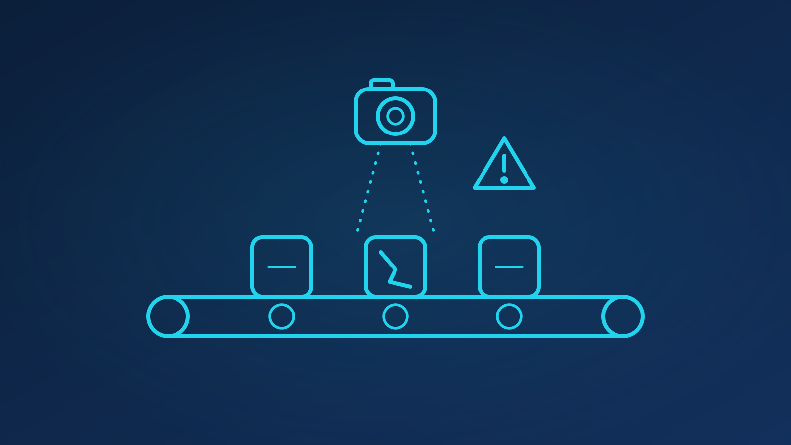
Computer vision defect detection works when the imaging is fixed before the model is chosen: consistent lighting and camera placement, a labelled set that reflects real production, a model matched to how rare the defects are, and inference at the edge fast enough to act on the line. Most failed projects did not fail on the algorithm; they failed on glare, unlabelled edge cases, or a false-positive rate that made operators switch the system off. This is the order of work we follow.
TL;DR
- Spend the first weeks on optics: lighting, lens, camera position and part presentation decide the ceiling of any model.
- Collect and label from real production, including the ugly edge cases, and agree what counts as a defect in writing.
- Use classical methods where defects are simple, supervised deep learning where they are varied, and anomaly detection where they are rare.
- Run inference at the edge with a latency budget derived from line speed, and integrate with the PLC through a defined signal.
- Model the economics of false positives versus escapes, then monitor drift and plan retraining from day one.
Why does lighting matter more than the model?
A defect the camera cannot see cannot be detected. Before any data science, someone has to answer: what defect classes are we looking for, how large are they, and what lighting makes them visible? Scratches on metal show under low-angle dark-field light; dents under diffuse dome lighting; contamination may need UV or infrared. Fix camera position, lens, exposure and working distance, shield the station from ambient light, and present the part in a repeatable pose.
Then check the basics that break later: resolution per millimetre against the smallest defect, motion blur at line speed (which sets shutter time and often demands a strobe), and an enclosure that keeps dust and vibration off the optics. Every hour here saves days of "the model is behaving oddly" that turns out to be a flickering tube.
How do you collect and label data that reflects production?
Capture from the actual station across shifts, batches and material lots. Aim for hundreds of good parts and as many defective ones as you can get, and log line, shift and lot for each so you can later test whether the model generalises.
Labelling needs a written definition of each defect class with example images, agreed with quality engineers, because "scratch versus mark" disagreements between labellers become model noise. Choose the label type by the decision you need: image-level pass/fail is cheapest; bounding boxes support localisation and counting; pixel masks are needed to measure defect area against a tolerance. Lock a held-out test set away from the start.
Classical, deep learning or anomaly detection?
The choice depends on how well defined and how frequent the defects are.
| Situation | Approach | Data needed | Strengths and limits |
|---|---|---|---|
| Simple, well-defined defects on stable parts (missing hole, wrong colour, dimension out of tolerance) | Classical CV: thresholding, edge detection, template matching, blob analysis | Tens of examples, mostly for tuning | Fast, explainable, no training; brittle to lighting change |
| Varied defects with plenty of labelled examples | Supervised deep learning (classification, detection or segmentation) | Hundreds to thousands per class | Handles variety and texture; needs labels and retraining |
| Defects rare or unpredictable | Anomaly detection trained on good parts only | Many good parts, few or no defects | Catches novel defects; explains less, threshold tuning matters |
| Mixed: mostly rare, some known classes | Anomaly detection to flag, supervised classifier to name | Both | Best coverage; two models to maintain |
On most lines defects are rare by design, so anomaly detection on good-part images is the usual starting point, with a supervised model added once enough labelled defects have accumulated. Fine-tuning a pretrained detector on a few hundred labelled images is a normal first milestone.
How fast does inference need to be, and where does it run?
Work back from the line. If parts pass at one per second and the reject mechanism sits 400 mm downstream, you have a hard budget for capture, inference and the reject signal. That usually rules out a cloud round trip and puts inference on an industrial PC or edge device beside the line. Quantised models in an optimised runtime often meet the budget where the training-time model would not.
Integration with the PLC is a signal contract, not an afterthought: a trigger in from the part-present sensor, a pass/fail or class code out over a fieldbus or digital I/O, a heartbeat so the PLC knows the vision system is alive, and a defined behaviour when it is not (fail-safe stop or fail-open with an alarm, agreed with the line owner). Every decision, image and score is logged locally and synced for review.
What do false positives cost, and how do you keep the model honest?
Two error types, two costs. A false positive rejects a good part: scrap or rework, plus operators learning to distrust the system. An escape passes a defective part: warranty, recall or complaint. Put money on both, then set the threshold to minimise the total rather than to maximise a headline accuracy. Where an escape costs a hundred times a false reject you accept more false rejects; on a cosmetic line the balance shifts the other way. Show operators why a part was rejected (a heatmap or box) so they can override with a reason, and treat overrides as labels.
Then plan for drift. Materials, suppliers, tooling wear and seasonal light all shift the image distribution. Monitor score distributions, reject rates and override rates per shift, alert when they move, and schedule retraining from newly labelled production data with the same held-out test set as the gate. That is the MLOps part of the job, and it is what keeps a system useful past its first month.
What does a sensible pilot look like?
Pick one station with a clear defect definition and a measurable cost, install the imaging and run it in shadow mode alongside the existing inspection for a few weeks so every decision is compared with the human outcome. Set the go-live criteria in advance: escape rate below the current process, false-reject rate the line can absorb, latency within budget, and operator acceptance. Only then connect the reject signal.
Illustratively, a well-run pilot moves from imaging design to shadow mode in a couple of months, and later stations go faster because the imaging templates, labelling guide and integration pattern already exist. If you are weighing up a first line, our computer vision team will look at sample images and say honestly whether it will work; get in touch.
Key takeaways
- Imaging determines the ceiling; fix lighting, optics and part presentation before touching a model.
- Label from real production with a written defect definition and a locked test set.
- Match the method to defect frequency: classical for simple, supervised for varied, anomaly detection for rare.
- Derive the latency budget from line speed, run at the edge and define the PLC signal contract including failure behaviour.
- Price false rejects against escapes to set the threshold, and monitor drift with retraining built in.
FAQ
How many defective examples do we need before starting?
Fewer than most teams fear. Anomaly detection can be trained on good parts alone and will flag unfamiliar defects with no defective examples at all. A supervised classifier or detector typically becomes useful with a few hundred labelled examples per defect class when built on a pretrained backbone. Start collecting from the real station immediately, because the images gathered during the imaging trials are already valuable training and evaluation data.
Can we use the cameras we already have on the line?
Sometimes, but check three things first: whether the resolution covers the smallest defect at the working distance, whether the shutter and lighting freeze motion at line speed, and whether you can control the lighting and exclude ambient light. Existing monitoring cameras often fail on lighting rather than resolution. A modest investment in a dedicated camera, lens and light usually pays back quickly in model performance and stability.
What happens when a new type of defect appears that the model has never seen?
An anomaly-detection model will usually flag it as unfamiliar, which is exactly why we recommend it as the first layer on lines where defects are rare. A purely supervised model may pass it. Either way, the operator override log and periodic sampling of passed parts should surface it; the new class is then defined, labelled and added at the next scheduled retraining, with the test set updated to include it.

Written by
Ali Waqas · Data Scientist
Owns data exploration, model development and evaluation, from forecasting and NLP to computer vision.
About the team →Related services
Ready to chart your AI course?
A free 30-minute consultation: we listen, ask hard questions and tell you honestly where AI will and won't help.